


Conditional Formatting Based on Another Cell in Excel
Conditional formatting in Excel is a powerful feature that allows you to format cells based on specific criteria. While this is often done based on the value of the cell you’re evaluating, there are situations where you need to apply conditional formatting to a cell based on the values in another cell or column. In this comprehensive guide, we’ll provide examples to demonstrate how to achieve this in Excel.
How to Format Cells Based on Another Column in Excel
Imagine you have a sales dataset with the following columns: Product, Sales, and Target. You want to use conditional formatting in Excel to highlight the products that have achieved or exceeded their sales target. Here’s how:
- Select the Sales column.
- Go to the Home tab, click on Conditional Formatting in the Styles group, and select New Rule. This opens the New Formatting Rule dialog box.
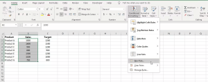
Image by https://www.makeuseof.com/ - In the New Formatting Rule dialog box, choose “Use a formula to determine which cells to format.”
- Enter the following formula in the “Format values where this formula is true” text box:
=B2 >= $C2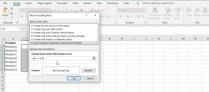
Image by https://www.makeuseof.com/ This formula checks if the value in column B (Sales) is greater than or equal to its corresponding target value in column C.
-
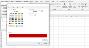
Image by https://www.makeuseof.com/ Click on the Format button to choose the formatting style you wish to apply to the cells that meet the condition, such as fill color, font color, etc.
- Click OK when you’re done. The formatting will now be applied to highlight the sales values that meet the specified condition.
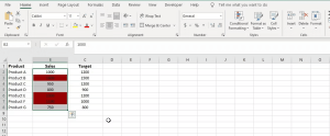
Image by https://www.makeuseof.com/
How to Format an Entire Column Based on a Cell Value in Excel
Now, let’s say you have a budget spreadsheet with the following columns: Category (column A) and Actual Expense (column B). You want to compare the actual expense with a budget limit specified in a specific cell (D2, for example), and highlight the cells in column B that exceed the budget limit. Here’s how:
- Select the entire Actual Expense column.
- Go to the Home tab in the Excel ribbon.
- Click on Conditional Formatting in the Styles group, and select New Rule. This opens the New Formatting Rule dialog box.
- In the New Formatting Rule dialog box, select “Use a formula to determine which cells to format.”
- Enter the formula below to check if each expense exceeds the budget limit in cell D2:
=$B2 > $D$2This formula checks if the value in each cell of column B exceeds the budget limit specified in cell D2.
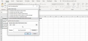
Image by https://www.makeuseof.com/ - Click on the Format button to define the formatting style you want to apply to expenses that exceed the budget limit.
- Click OK to close the Format Cells dialog box.
- Click OK again in the New Formatting Rule dialog box.
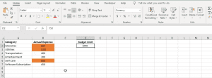
Image by https://www.makeuseof.com/
Now, whenever you change the value in cell D2 (or any cell used in the formula), the formatting will adjust automatically and highlight the categories that exceed the new budget limit.
Comparative Table: Formatting Techniques
Let’s summarize the two conditional formatting techniques we’ve covered in this guide for quick reference:
| Technique | Use Case | Steps |
|---|---|---|
| Formatting Cells Based on Another Column | Highlight specific cells based on values in a different column. | 1. Select the target column.<br />2. Go to Conditional Formatting > New Rule.<br />3. Use a formula to determine formatting based on another cell’s value.<br />4. Define formatting style. |
| Formatting an Entire Column Based on a Value | Format an entire column based on a value in a single cell. | 1. Select the entire column.<br />2. Go to Conditional Formatting > New Rule.<br />3. Use a formula to determine formatting based on a specific cell’s value.<br />4. Define formatting style. |
Conclusion
Conditional formatting in Excel is a versatile tool that can significantly enhance your data presentation and analysis. While it’s commonly used to format cells based on their own values, the ability to format cells based on values in other cells or columns opens up a world of possibilities for more dynamic and insightful spreadsheets. By mastering these techniques, you can take control of your Excel spreadsheets, making them more efficient and visually engaging. Whether you’re managing budgets, tracking sales targets, or analyzing any type of data, conditional formatting can save you time and help you make informed decisions.