


Google Sheets Quick Hacks You Probably Didn’t Know
Google Sheets has long been your trusty spreadsheet tool for managing data. But did you know that it’s not just about columns and formulas? Google Sheets harbors a treasure trove of hidden features and hacks that can revolutionize the way you work, both professionally and personally. In this article, we’re going to unveil the top 10 Google Sheets hacks that you probably didn’t know existed, and how they can add convenience and innovation to your life.
1. Creating QR Codes
QR codes can be handy for various purposes, such as tracking attendance or sharing information. In Google Sheets, you can generate QR codes easily using the following formula:
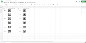
=IMAGE("https://chart.googleapis.com/chart?chs=200x200&cht=qr&chl="&A2&")")
Here’s how it works:
=IMAGE(): This function inserts an image into a cell."https://chart.googleapis.com/chart?chs=200x200&cht=qr&chl="&A2&"": This part constructs a URL for generating a QR code. It combines a fixed part of the URL with the content from cellA2, which can be any data you want to encode in the QR code.
Replace A2 with the cell reference containing the data you want in the QR code. When you enter this formula in a cell, it will display the QR code corresponding to the data in that cell.
2. Image URLs
Managing images in Google Sheets becomes more convenient with this hack. Instead of manually inserting images, you can use formulas to fetch them from the internet. Here’s how:
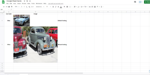
=IMAGE("url")
=IMAGE(): This function displays an image in a cell."url": Replace this with the online link to your image.
You can also customize the image’s dimensions and alignment as per your needs. This is particularly useful for social media enthusiasts, web developers, and bloggers who frequently work with images.
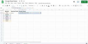
3. Randomizing Names and Numbers
Randomizing names or numbers is useful for things like lucky draws or team assignments. In Google Sheets, you can do this easily:
- List the names in a column.
- In an adjacent cell, use this formula:
=CHOOSE(RANDBETWEEN(1,6),A2,A3,A4,A5,A6,A7)
=CHOOSE(): This function selects a value from a list based on its position.RANDBETWEEN(1,6): This generates a random number between 1 and 6 (adjust the range as needed).A2, A3, A4, A5, A6, A7: These are the names you want to choose from. Adjust the range to match your list.
Whenever you recalculate your sheet or press Enter in the cell with this formula, it will randomly pick one name from the list. This ensures fairness in selections or giveaways.
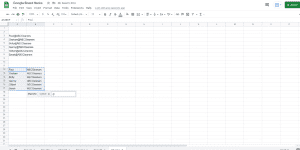
4. Create a Drop-Down List
Drop-down lists are handy for data input and selections. Here’s how to create one:
- Select a cell where you want the drop-down list.
- Go to
Data>Data validation. - Under
Criteria, selectList of items. - In the
List of itemsfield, input the items you want in the drop-down list, separated by commas.
Now, when you click on the cell, a drop-down arrow will appear, allowing you to choose from the predefined items. This is great for surveys, quizzes, or creating menus.
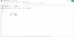
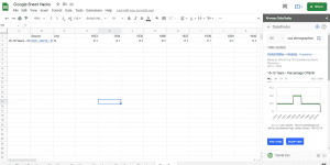
5. Download Data
You can import data from websites directly into your Google Sheets. Here’s how:
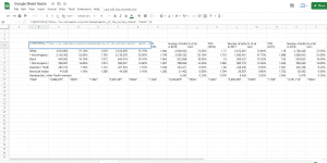
- In any cell, use the formula:
=IMPORTHTML("https://en.wikipedia.org/wiki/Demographics_of_the_United_States","table",4)
"https://en.wikipedia.org/wiki/Demographics_of_the_United_States": Replace this with the URL of the webpage you want to import data from."table": Specifies that you want to import a table from the webpage.4: Indicates which table on the webpage to import (you can adjust this number as needed).
Upon pressing Enter, data from the specified webpage’s table will be loaded directly into your worksheet.
6. Self-Checking Assessments
You can use Google Sheets’ Conditional Formatting to create self-checking question papers or assessments. Here’s how:
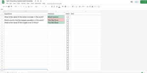
- Input your questions and answers in separate sheets. For example, questions go in one sheet, and answers go in another.
- Hide the sheet containing the answers.
- In the question sheet, use conditional formatting to compare the answers given by students with the hidden correct answers. When students input their answers, conditional formatting can highlight correct and incorrect responses, providing instant feedback.
This is particularly useful for self-assessment or practice quizzes, allowing students or users to gauge their understanding immediately.
7. CLEAN and TRIM Functions
Google Sheets provides two functions, CLEAN and TRIM, to help you clean up and format your data:
- CLEAN: This function removes all unprintable characters from text. It’s handy when dealing with data that might have hidden characters or formatting issues.
- TRIM: TRIM removes unnecessary spaces at the beginning or end of a text string. It’s useful when you have data with extra spaces, which can affect sorting and filtering.
Both functions can save you a lot of manual effort when working with messy data in your spreadsheets.
8. Split Data
Splitting text into different columns is common when dealing with datasets that need reformatting. Doing this manually for large datasets can be time-consuming. Here’s how to do it efficiently:
- Select the entire data that you want to split into two columns.
- Go to
Datain the menu bar and then selectSplit text to columns. - Choose the appropriate separator, or you can even select a custom character that separates the text.
Google Sheets will split the text based on your chosen separator, saving you the time and effort of doing it manually.
9. Visualize All Keyboard Shortcuts
Keyboard shortcuts can significantly boost your productivity in Google Sheets. To access a list of all keyboard shortcuts:
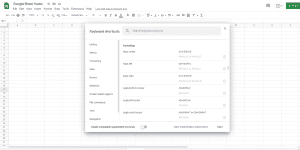
- Press
Ctrl + /on Windows orCommand + /on macOS.
This keyboard shortcut will bring up a list of Google Sheets keyboard shortcuts on your screen, making it easy to reference them as you work. It’s a handy way to quickly learn and start using keyboard shortcuts to navigate and manipulate your spreadsheets more efficiently.
10. Find Related Data
When creating reports or gathering data, finding the right information can be time-consuming. Instead of manually searching, you can use data finder add-ons for Google Sheets. Here’s how:
- Install a data finder add-on, such as Knoema DataFinder, in your Google Sheets.
- Bookmark data that you frequently use in the add-on.
- When creating a report, open the add-on, and easily insert the bookmarked data into your report.
These add-ons can save you valuable time by streamlining the process of finding and inserting relevant data into your documents.
| Google Sheets Hack | Description |
|---|---|
| 1. Creating QR Codes | Generate QR codes for various purposes, such as tracking employee attendance, student check-ins, or event participants, directly within Google Sheets using a simple formula. |
| 2. Image URLs | Easily manage images by fetching them from the internet using a formula, saving time on manual updates. |
| 3. Randomizing Names and Numbers | Fairly select names or numbers at random using the RANDBETWEEN formula, useful for giveaways or team selections. |
| 4. Create a Drop-Down List | Enhance data input accuracy by adding drop-down lists, ideal for surveys, quizzes, and menu creation. |
| 5. Download Data | Import data from websites directly into your spreadsheet using the IMPORTHTML formula. |
| 6. Self-Checking Assessments | Use Conditional Formatting to create self-checking question papers or assessments, providing instant feedback for users. |
| 7. CLEAN and TRIM Functions | Clean up data by removing unprintable characters with the CLEAN function and eliminate unwanted spaces with the TRIM function. |
| 8. Split Data | Efficiently split text into two columns with the Data > Split text to columns feature. |
| 9. Visualize All Keyboard Shortcuts | Quickly access and memorize all Google Sheets keyboard shortcuts by pressing Ctrl + / (Windows) or Command + / (macOS). |
| 10. Find Related Data | Save time searching for data by using data finder add-ons like Knoema DataFinder to easily insert bookmarked data into your reports. |
This table provides a concise overview of each Google Sheets hack, making it easy for readers to understand and reference the key points. You can also format it in your article to make it visually appealing to your audience.
Conclusion
Google Sheets is a versatile tool that goes beyond the basics of spreadsheets. These ten hacks are here to help you take full advantage of its capabilities, making your professional and personal life more efficient and enjoyable.
These hacks are not only easy to learn but also add innovation to your daily tasks. They empower you to work smarter, not harder, whether you’re a student, professional, or just someone looking to make life a bit more efficient.
So, why wait? Start implementing these Google Sheets hacks today and supercharge your experience with this powerful spreadsheet tool. Enjoy the convenience and creativity they bring to your projects, and watch as your productivity soars. Happy Google Sheets hacking!